Jag har gjort två kartor över allmännyttan i Stockholms stad 2007-2013. Här följer en arbetsbeskrivning.
Insamling av data
Kartorna bygger på fastighetsförteckningar från bostadsbolagens årsredovisningar. Årsredovisningarna finns att ladda ner i pdf-format på respektive bolags hemsida. Jag använde mig av programmet pdftk för att “klippa ut” de sidor jag ville ha från årsredovisningen, det vill säga endast fastighetsförteckningen.
Programmet körs i terminalen på Linux, och jag använde följande kommando:
pdftk arsredovisning.pdf cat 34-46 output fastighetslista.pdf
Det säger åt pdftk att ta ut sidorna 34-46 från filen arsredovisning och skriva ut till en ny fil, fastighetslista. Med hjälp av sidan Cometdocs omvandlade jag sedan pdf-filerna till xls-filer.
Städning av data
Xls-filerna krävde en hel del städning. Jag använde Open Refine för att bland annat ta bort onödiga kolumner och text. I Libre Office Calc lade jag till kolumner som saknades och skapade ett fullständigt adressfält. Till sist slog jag ihop filerna från de olika bostadsbolagen till en enda fil för varje år. Resultatet blev sju filer med cirka 1500 rader i varje.
I Libre Office Calc var formeln VLOOKUP till väldigt stor hjälp. I två av fastighetsförteckningarna fanns det inga gatunummer, utan bara gatunamn. Genom VLOOKUP kunde jag “hämta” många adresser från ett annat års förteckning. Sedan kompletterade jag de adresser som inte fanns med där genom att söka på nätet.
Geokodning
Först installerade jag ett litet script i Google Docs Spreadsheet, enligt instruktioner på denna sida: http://schoolofdata.org/handbook/recipes/geocoding/. Det klarade inte att geokoda alla adresser.
I ett senare läge visade det sig också att det gav samma koordinater till adresser med samma gata, fast olika gatunummer. Det ledde till ett stort fel på kartan, eftersom flera fastigheter blev en och samma punkt. Därför använde jag även gpsvisualizer.com/geocoder för många av adresserna.
Visualisering
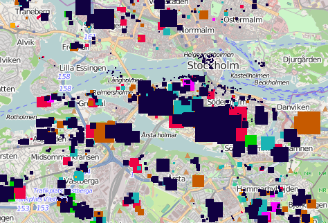
Kartan är gjord med hjälp av OpenLayers, som är ett open source Javascript-bibliotek för att skapa kartor. Jag kopierade koden på denna länk: http://wiki.openstreetmap.org/wiki/Openlayers_POI_layer_example och sparade xls-filerna som csv-filer enligt mallen på samma sida.